Tensors all the way down
I’ve trained a lot of neural networks in PyTorch. Autograd is a wonderful invention… and also a wonderful way to completely lose track of what your model is actually doing. Somewhere under the loss.backward() call, there’s a stack of matmuls, a couple nonlinearities, and a loop quietly walking those same tensors backward.
In an effort to deepen my intuition on neural nets, I built a fully connected MNIST classifier in raw NumPy. No PyTorch, TensorFlow, or autograd. The architecture itself is tiny on purpose, that’s not really the point. Once you write a layer as \(WA + b\), adding another layer just means appending another pair of tensors. Two layers, twenty layers, it doesn’t really matter, it’s still the same program.
The notebook is here if you want to see the code.
Problem statement
MNIST is the “hello world” of image classification: 28×28 grayscale handwritten digits, labeled 0 through 9.
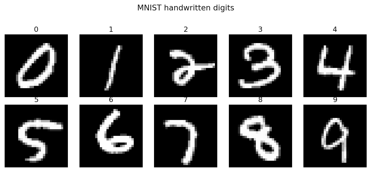
Each image is just 784 numbers. One per pixel, from 0 (black) to 255 (white). We want to turn those 784 numbers into a guess over the ten digits. I used 42,000 labeled examples from the Kaggle Digit Recognizer set, shuffled them, split 80 / 10 / 10 into train, validation, and test (33,600 / 4,200 / 4,200), and divided every pixel by 255 so the inputs live in \([0, 1]\).
In the math below, a batch of images is a matrix \(X \in \mathbb{R}^{784 \times m}\): each column is one flattened digit. Most libraries do the opposite (rows as examples). Column-as-example is the whiteboard convention, because then a layer really is \(Z = WX + b\) instead of \(Z = XW^\top + b^\top\). I transpose the CSV once and don’t think about it again.
A tiny network
The network I trained looks like this:
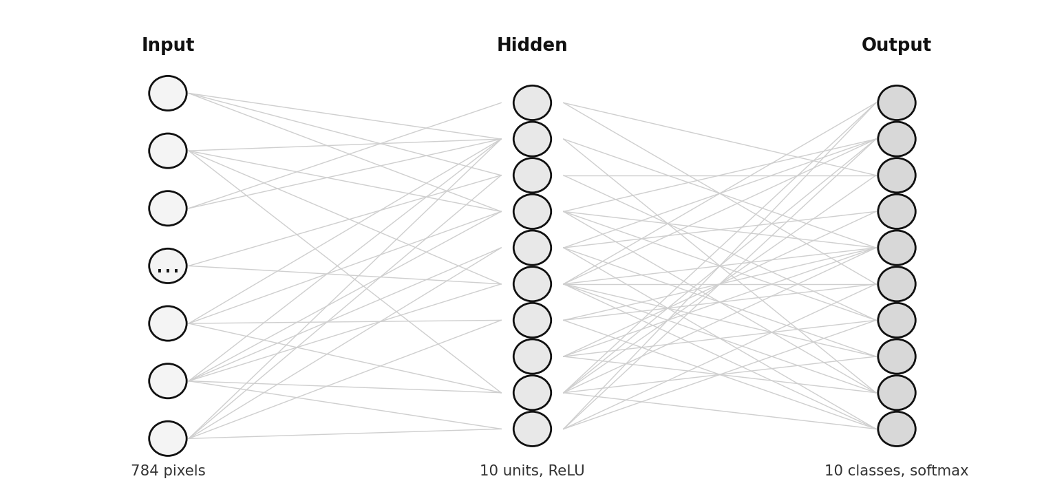
- Input: 784 nodes, one per pixel.
- Hidden layer: 10 nodes. Mix the pixels together, then ReLU.
- Output: 10 nodes, one per digit. Mix the hidden layer, then softmax, so the ten scores become a probability distribution.
Because the input has no weights of its own, this is a two-layer network. Between layer \(l-1\) and layer \(l\), the weights are \(W^{[l]} \in \mathbb{R}^{n^{[l]} \times n^{[l-1]}}\) and the bias is \(b^{[l]} \in \mathbb{R}^{n^{[l]} \times 1}\). For this net that means \(W^{[1]}\) is \(10 \times 784\), \(W^{[2]}\) is \(10 \times 10\), and both biases are \(10 \times 1\).
The implementation never hardcodes “two.” It takes a list of layer sizes ([784, 10, 10] here) and builds a Python list of those \((W, b)\) pairs. Swap in [784, 64, 32, 10] and you’d train a deeper net with the same loop. Weights start as small random numbers, uniform in \([-0.5, 0.5]\).
Going forward
Start with \(A^{[0]} = X\). For each layer:
\[Z^{[l]} = W^{[l]} A^{[l-1]} + b^{[l]}\] \[A^{[l]} = g^{[l]}(Z^{[l]})\]\(Z^{[l]}\) is the pre-activation: a linear mix of the previous layer. The bias is \(n^{[l]} \times 1\), but it broadcasts across all \(m\) columns, which is exactly “add this vector to every example.”
If you stacked two of those with nothing in between, they’d collapse into a single linear map and just become a very advanced linear regression:
\[W^{[2]}(W^{[1]} X + b^{[1]}) + b^{[2]} = (W^{[2]} W^{[1]}) X + \ldots\]The activation is actually what makes a layer worth having by introducing nonlinearity.
Hidden layers use ReLU, which is extremely simple: it passes positive values through and turns negatives off.
\[\text{ReLU}(z) = \max(0, z)\]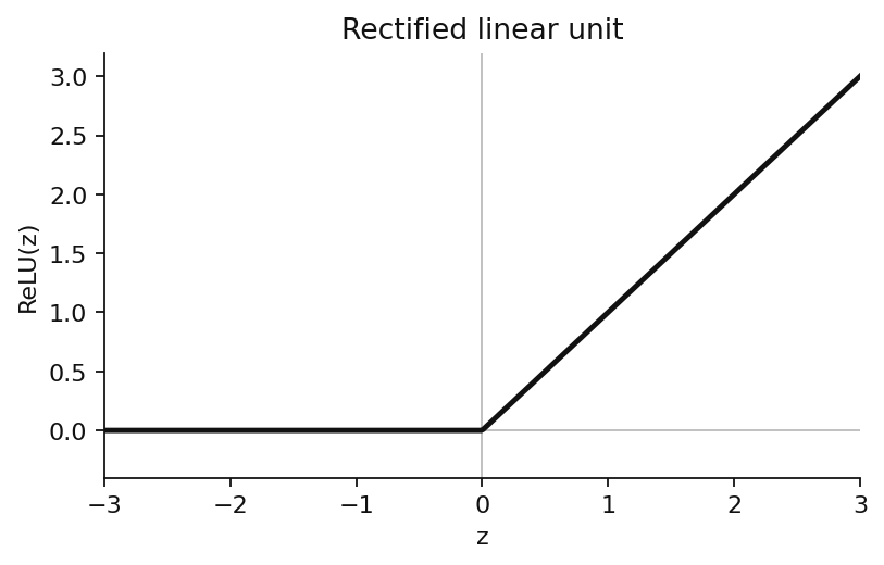
That kink at zero is enough. The function is easy to differentiate, and it keeps the whole network from flattening into one big matrix multiply.
The last layer uses softmax, which turns raw class scores into a probability distribution: positive numbers that sum to 1.
\[\text{softmax}(z)_i = \frac{e^{z_i}}{\sum_k e^{z_k}}\]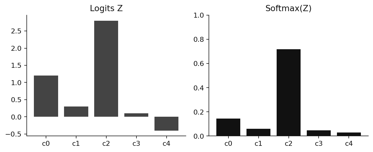
You can read \(A^{[L]}_{i,j}\) as “the model’s probability that example \(j\) is digit \(i\).” The predicted digit is whichever class got the biggest share. In the implementation, subtract the per-column max before exponentiating — softmax doesn’t care about a constant shift, and that keeps exp from overflowing when logits get large.
So a forward pass here is: multiply-and-add, ReLU, multiply-and-add, softmax. One linear step per layer, with softmax only at the very end.
Going backward
A random network is a random guesser. Training is nudging the weights so the probabilities line up with the true labels.
The usual way to measure that mismatch is cross-entropy. If \(\hat{y}\) is the predicted distribution and \(y\) is a one-hot vector for the true digit:
\[J(\hat{y}, y) = -\sum_{i=0}^{9} y_i \log \hat{y}_i\]The sum collapses to a single term, \(-\log \hat{y}_{\text{correct}}\). Probability 0.8 on the right digit is a loss of about 0.22; probability 0.01 is about 4.6. If the model puts high probability on the correct digit, the loss is small; if it’s wrong and confident, the loss blows up.
Gradient descent then asks, for every weight, “which way should I step to make that number smaller?” and takes a small step that way, over and over.
\[W^{[l]} \leftarrow W^{[l]} - \alpha \frac{\partial J}{\partial W^{[l]}}\]\(\alpha\) is the learning rate — here, 0.10 — a parameter we pick rather than something the model learns.
Computing those derivatives by hand sounds (and is) grim, but backprop is just the chain rule run in reverse. You start from how wrong the output was and push that error backward through the same weights that produced it. Softmax plus cross-entropy has a gift: the two derivatives collapse into a subtraction. If \(Y\) is the one-hot matrix of labels and \(A^{[L]}\) is the softmax output,
\[dZ^{[L]} = A^{[L]} - Y\]That’s the entire error signal at the last layer. Then, walking backward, each layer is the same three lines:
\[dW^{[l]} = \frac{1}{m}\, dZ^{[l]}\, A^{[l-1]\top}\] \[db^{[l]} = \frac{1}{m} \sum_j dZ^{[l]}_{:,j}\] \[dZ^{[l-1]} = \big(W^{[l]\top} dZ^{[l]}\big) \odot \text{ReLU}'(Z^{[l-1]})\]A few facts make this less mysterious than it looks:
- \(dW^{[l]}\) is (in batch form) an outer product of this layer’s error with the previous layer’s activations. A connection grows when the incoming neuron was active and the outgoing one was wrong.
- The \(1/m\) averages over the batch, so the gradient doesn’t silently scale with dataset size.
- \(W^{[l]\top} dZ^{[l]}\) is the forward map run in reverse: error at layer \(l\), pushed back onto layer \(l-1\) through the same weights.
- ReLU’s derivative is a mask: 1 if \(z > 0\), else 0. Units that were off on the way forward don’t get a vote on the way back.
Do that for every layer, step the weights, and that’s one iteration of training. I used full-batch gradient descent — every update sees all 33,600 training examples at once — because the path is smoother and it’s easier to tell whether the gradients are actually correct. Mini-batches would be the more common (and usually faster) choice.
Forward, backward, step. 500 times, layer_sizes=[784, 10, 10], \(\alpha = 0.10\). That’s the whole algorithm.
What it learned
From chance to “mostly reads digits” in a few hundred passes:
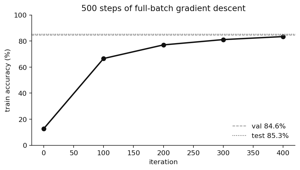
Training accuracy went 12.7% → 66.6% → 77.0% → 81.1% → 83.4% at iterations 0 / 100 / 200 / 300 / 400. After 500 iterations, validation accuracy was 84.6% and test accuracy was 85.3%. A random guesser sits at 10%. A well-tuned CNN on MNIST sits above 99%. This model has ten hidden units, no convolutions, no data augmentation, and vanilla gradient descent, so the mid-80s seems about right: it has learned something real about digit shapes, and it has also hit the ceiling of a network this small.
After poking into failure modes, I found that it’s usually the obvious human confusions, like a 4 that looks like a 9, a 3 that leans toward a 5. Ten hidden units have to compress 784 pixels into a tiny code, so there’s only so much handwriting variation they can spend capacity on.
Why write this in 2026
None of this is “useful” by modern standards, obviously. Modern PyTorch/Tensorflow fuses the matmuls, runs them on a GPU, hands you Adam for free. Doing it by hand definitely resulted in a worse classifier, but it gave me a better understanding of what’s going on under the hood.
There’s a lot of room to expand on this — mini-batches, decent initialization, Adam, more hidden units, convolutions. Maybe something for a future blog post :P